Article History

Published: Fri 11, Apr 2025
Received: Tue 11, Feb 2025
Accepted: Tue 18, Mar 2025

View PDF

Download PDF

Author Details

Fan Yang Hongliang Zou Jiaxiong Xie

Abstract

Autophagy proteins (ATGs) play a vital role in the human body, and abnormalities in ATGs degradation have been linked to various illnesses, including neurological diseases, cancer, and cardiovascular disease. Therefore, accurately predicting ATGs from a large pool of non-ATGs is a pressing task in the post-genome era. To address this issue, we have developed a novel computational model called ATG-Pred to discriminate ATGs from non-ATGs in this study. Initially, we employed the residue pairwise energy content to encode the protein sequences. Furthermore, to get important information, both auto-covariance and cross-covariance were used. To remove irrelevant and redundant characteristics, we used the analysis of variance (ANOVA) approach. After that, the features that were chosen were fed into a support vector machine so that it could be used to distinguish between ATGs and non-ATGs. In the jackknife test, our method achieved classification accuracies of 95.17% and 96.50% on the training and test dataset, respectively. Moreover, compared to current state-of-the-art methods, our proposed approach has shown enhanced classification performance, confirming its efficacy in identifying ATGs. For the convenience of academic use, we have made the codes and datasets used in our study available at (Link 1).

Keywords

Autophagy proteins, residue pairwise energy content, auto- and cross-covariance, support vector machine, jackknife test

1. Introduction

Autophagy, a crucial cellular process that maintains cell homeostasis and regulates cellular energy metabolism [1], plays a pivotal role in various biological process. Dysfunctions in autophagy have been linked to some serious illnesses, such as neurodegenerative diseases, cancer, and aging [2-5]. Importantly, the crucial role of autophagy in biomedical science was acknowledged by the Nobel Prize in Physiology or Medicine in 2016 [6]. Many studies have emphasized the role of various autophagy proteins (ATGs) in regulating autophagy. For example, ATG9, the sole known ATG membrane protein, alongside ATG2 and ATG15, forms a recycling system that provides lipid membranes necessary for autophagosome production and growth [7, 8]. Consequently, distinguishing ATG proteins from non-ATGs proteins has become an urgent task in the post-genome era. While experimental methods are considered the most reliable ways to unveil the biological functions of ATGs, they can be time-consuming and expensive. Accordingly, in recent years, machine learning approaches have gained attention due to their efficiency and convenience. In the bioinformatics area, several computational models have been developed for exploring peptides, proteins, DNA, and RNA [9-21].

In an effort to discriminate ATGs from non-ATGs, Jiao and colleagues constructed the first machine learning model called ATGPred-FL to study this issue [22]. This predictor employed three different feature methods to encode protein sequences, namely amino acid composition features, physicochemical property-based features, and sequence order-based features. To enhance the informative nature of probability features, a feature learning method was used. Furthermore, a two-step feature selection strategy was used to select the best feature subset, with support vector machine serving as the classifier for ATGs identification. It was noted that there were 94.40% and 90.50% classification accuracies for each of the training and test dataset, respectively, for which this predictor was able to do so.

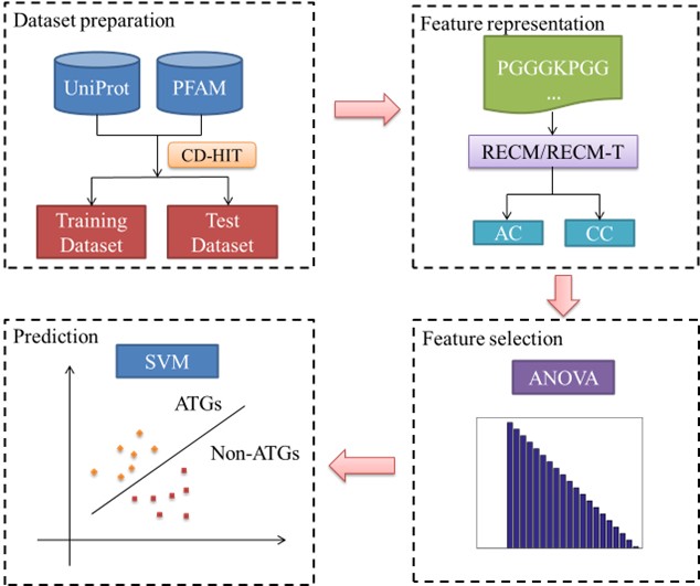
While ATGPred-FL has shown encouraging results in predicting ATGs, there are still some unresolved difficulties that need to be solved in future studies. One such issue is the lack of consideration for correlation attributes among different features in ATGPred-FL. To tackle this challenge, our study introduces a feature fusion algorithm called similarity network fusion (SNF) to integrate diverse features. To determine the optimal feature combination, we implement the analysis of variance (ANOVA) approach. These chosen features are then utilized as input for the support vector machine to distinguish between ATGs and non-ATGs. To further illustrate the proposed method, we have included (Figure 1), which provides a visual representation of the process. In the next sections, we shall give a full explanation of each component depicted in the figure.

2. Materials and Methods

2.1. Datasets

Using the same dataset as in a previous work [22], we performed this work. With the same data used in this way, we were able to directly compare the performance of our proposed method with that of the state-of-the-art method to the current one. To ensure a rigorous evaluation of our developed model, we divided the dataset into training and test datasets. There were 393 positive samples (i.e., ATGs) and 393 negative samples (i.e., non-ATGs), in the training dataset. Conversely, the test dataset consists of 200 samples, with 100 positive samples and an equal number of negative samples. The positive samples were collected from the Universal Protein Knowledge Base (UniProtKB) [23], while the negative samples were obtained from the protein family database (PFAM) [24]. To ensure diversity in the dataset, we ensured that any two sequences within the same subgroup had no more than 85% sequence identify, which was achieved using the CD-HIT toolbox [25].

2.2. Feature Representation

In this study, we utilized the residue pairwise energy content matrix (RECM) [26] to extract informative classification features from the protein sequences. The RECM was calculated by using least squares regression to fit the residue pairs of the tertiary structure of the 785 proteins to main sequence of 674 proteins, which was obtained by the RECM. The RECM has demonstrated its effectiveness in protein and peptide prediction [27, 28]. Based to the concept, the RECM is a 20×20 matrix derived from experimental techniques. Therefore, a protein with L amino acids can be effectively represented as follows:

\[\text { RECM }-T=\left[\begin{array}{cccc}p_{1,1} & p_{1,2} & \cdots & p_{1,20} \\p_{2,1} & p_{2,2} & \cdots & p_{2,20} \\\vdots & \vdots & \vdots & \vdots \\p_{L, 1} & p_{L, 2} & \cdots & p_{L, 20}\end{array}\right]\ \ \ \ (1)\]

where the i-th row in RECM-T matrix is the corresponding elements of i-th residue in the RECM matrix. For example, let’s examine a protein sequence P, which is comprised of the amino acids ‘ARNGG’. In this case, we would choose the corresponding row of ‘A’, ‘R’, ‘N’, ‘G’, ‘G’ from the RECM matrix. By doing so, we obtain a 5×20 matrix that effectively represents the sequence.

Next, it is crucial to extract useful information from this matrix for the classification task. In this study, we employed auto- and cross-covariance to select discriminative features. The auto-covariance (AC), in particular, can be expressed in the following mathematical form [29].

\[A C_{j, \lambda}=\frac{1}{L-\lambda} \sum_{i=1}^{L-\lambda}\left(p_{i, j}-\overline{p_j}\right)\left(p_{i+\lambda_{, j}}-\overline{p_j}\right)\ \ \ \ (2)\]

\[where\ \overline{p_j}=\frac{1}{L} \sum_{i=1}^L p_{i, j}.\]

Analogously, the cross-covariance (CC) can be mathematically represented as follows:

\[C C_{i_1, i_2, \lambda}=\frac{1}{L-\lambda} \sum_{i_1, i_2=1}^{L-\lambda}\left(p_{i_1, j}-\overline{p_{i_1}}\right)\left(p_{i_2, j+\lambda}-\overline{p_{i_2}}\right) \quad\left(i_1 \neq i_2\right)\ \ \ \ (3)\]

Indeed, the selection of parameter λ plays a vital role in capturing valuable information and obtaining reliable results. To cover a variety of options and to guarantee thorough coverage of helpful information from the matrix, in this paper, we took into consideration three different values for λ, namely 10, 15, and 20. In order to fully leverage the correlation information among different features, we incorporated the similarity network fusion algorithm [30]. This algorithm enabled us to integrate the features obtained from AC and CC for each value of λ. Consequently, three different feature matrices were generated, denoted as W¹, W² and W³, and corresponding to the λ values of 10, 15, and 20, respectively. According to the concept of SNF, a sparse matrix was initially obtained for Wⁱ(i= 1, 2, 3), and it can be defined as follows:

\[S^i(u, v)=\left\{\begin{array}{c}W^i(u, v), \text { if } v \in \delta_u \\0, \text { otherwise }\end{array}\right.\ \ \ \ (4)\]

where u and v represent two different rows in the feature matrix Wⁱ, and δu denotes the set of K nearest neighbors of u. The next step involves integrating the different features using an iterative approach, which can be calculated using the following formula:

\[\left(W^i\right)^{M+1}=S^i \times \frac{\sum_{j=1, j \pm i}^N\left(W^j\right)^M}{N u m} \times\left(S^i\right)^T\ \ \ \ (5)\]

where (W^J)^M represents the updated matrix Wⁱ after M iterations, Num refers to the number of matrices used for fusion, and in this study, the value of Num is 3. The notation T denotes matrix transposition. After the iterative process, we obtain the fused matrix by averaging the Num matrices as follows:

\[\bar{W}=\frac{1}{N u m} \sum_{i=1}^N W^i\ \ \ \ (6)\]

2.3. Feature Selection

In situations where the number of features exceeds the number of samples, noise, irrelevant information, and redundant features may be present, potentially impacting performance. To mitigate these issues, we adopted a widely-used feature selection approach known as the analysis of variance [31-34] to identify the most discriminative features. The following is the definition given to the F value of the k-th feature [31]:

\[F_k=\frac{s_B^2(k)}{s_W^2(k)}\ \ \ \ (7)\]

where \( s_B^2(k) \) indicates the sample variance between groups and \( s_W^2(k) \) represents the sample variance within groups. The following formula can be used to get these values:

\[s_B^2(k)=\frac{1}{d f_B} \sum_{i=1}^{K K} n_i\left(\frac{\sum_{j=1}^{n_i} f_{i j}(k)}{n_i}-\frac{\sum_{i=1}^{K K} \sum_{j=1}^{n_i} f_{i j}(k)}{\sum_{i=1}^{K K} n_i}\right)^2\ \ \ \ (8)\]

\[s_W^2(k)=\frac{1}{d f_W} \sum_{i=1}^{K K} \sum_{j=1}^{n_i}\left(f_{i j}(k)-\frac{\sum_{i=1}^{K K} \sum_{j=1}^{n_i} f_{i j}(k)}{\sum_{i=1}^{K K} n_i}\right)^2\ \ \ \ (9)\]

In this context, df_B = KK-1 and df_W = N-KK, KK indicates the number of groups, while N represents the total number of samples. F_ij (k) represents the frequency of the k-th feature in the j-th sample of the i-th group. Meanwhile, while simultaneously n_i indicating the total number of samples contained in the i-th group.

2.4. Support Vector Machine

In a number of biological researches, including proteins, peptides, DNA, and RNA [35-38], support vector machine is a potent machine learning algorithm with success. The core principle of SVM involves transforming raw data into a high dimensional feature space, where it aims to identify a hyper-plane that maximizes the margin to effectively separate samples from different classes. In the study, we implemented SVM with a radial basis kernel function (RBF) to perform the experiments. The choice of RBF kernel is based on the suitability of SVM in addressing small sample size issues, which is particularly relevant in our study.

2.5. Performance Evaluation

Accuracy (Acc), sensitivity (Sn), specificity (Sp), and Matthew’s correlation coefficient (MCC) were the four most often used metrics in the binary classification task to assess the performance of our classification model. These definition of these metrics are as follows [12, 39-42].

\[\left\{\begin{array}{c}S n=\frac{T P}{T P+F N} \times 100 \% \\S p=\frac{T N}{T N+F P} \times 100 \% \\A c c=\frac{T P+T N}{T P+F P+T N+F N} \times 100 \% \\M C C=\frac{T P \times T N-F P \times F N}{\sqrt{(T P+F P) \times(T N+F N) \times(T P+F N) \times(T N+F P)}}\end{array}\right.\ \ \ \ (10)\]

where TP is true positive, FP is false positive, TN is true negative, and FN is false negative. Additionally, to assess the overall performance, we calculated the area under the receiver operating characteristic (ROC) curve (AUC), which serves as a primary quantitative indicator.

3. Results and Discussion

3.1. Parameters Setting

In SVM with RBF, there are two parameters that need to be considered: the regularization parameter C and kernel parameter γ. To determine the optimal combination of these two parameters, we employed a grid search strategy. For parameter C, there were between 2^-5 and 2¹⁵ in the search space, with a step size of 2². Similarly, the search space for parameter γ ranged from 2^-15 to 2³, with a step size of 2^-2. Following a comprehensive review process, we determined that following parameters were used to get the best classification accuracy, these were set as follows:

\[\left\{\begin{array}{c}C=2^1, \gamma=2^{-1}, \text { forthetrainingdataset } \\C=2^3, \gamma=2^1, \text { forthetest dataset }\end{array}\right.\ \ \ \ (11)\]

3.2. Sequence Analysis

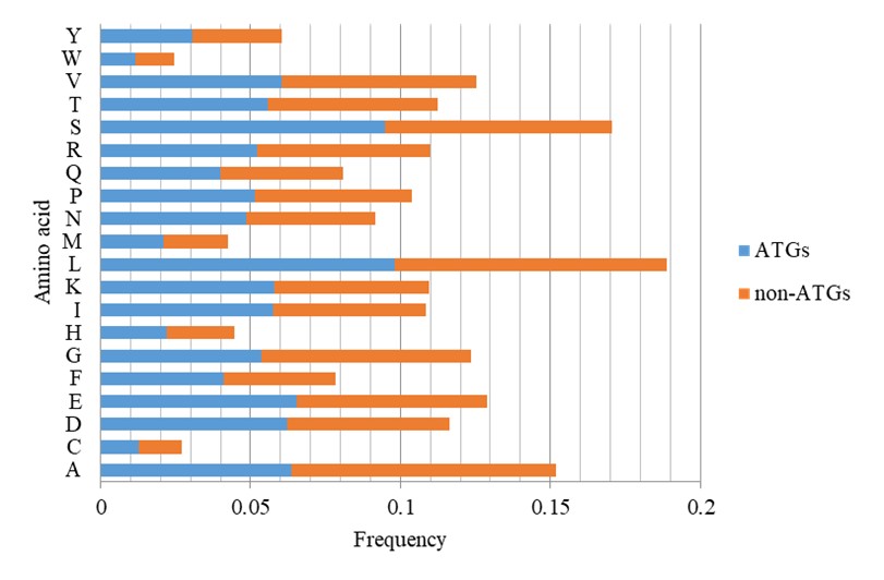
Figure 2 illustrated the discrepancy in amino acid frequencies between ATGs and non-ATGs sequences. By comparing the two groups, we see a considerable variation in the preferences of these two groups. For instance, non-ATGs exhibit a higher abundance of alanine and glycine, while ATGs display a greater prevalence of leucine and serine. These observations provide valuable insights that may serve as important clues in studying ATGs.

3.3. Classification Performance

Table 1 presents the classification results of the proposed method on the training and test datasets using jackknife test, while (Figure 3) displays the corresponding ROC curves. The table displays encouraging classification outcomes obtained through the proposed method. Specifically, the classification accuracy reached 95.80% and 97.00% on the training and test dataset, respectively. Additionally, the proposed method also obtained satisfactory results for the other four metrics.

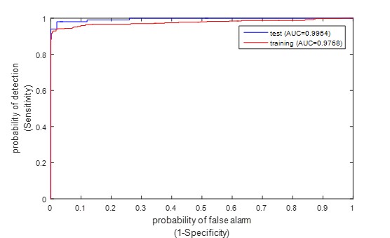
TABLE 1: The proposed method’s classification performance on the training and test datasets.

Dataset	Acc (%)	Sn (%)	Sp (%)	MCC	AUC
Training Test	95.80 97.00	92.11 96.00	99.49 98.00	0.9185 0.9402	0.9768 0.9954

3.4. Feature Visualization by t-SNE

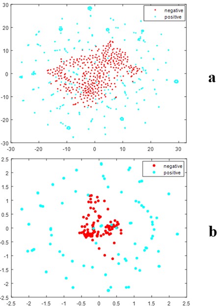
In this study, we employed a feature fusion strategy to integrate three types of features, and the ANOVA was utilized to select discriminative features. To verify the effectiveness of these selected features in classifying ATGs from non-ATG, t-SNE visualization was conducted. Figure 4 illustrates the distribution of feature space between positive and negative samples in a two-dimensional context. It can be seen from this figure that there was obvious separation between the distribution of positive and negative samples, this is not difficult to find. It may partly explain the powerful ability of our method in predicting ATGs as listed in (Table 1).

3.5. Influence of Parameter K

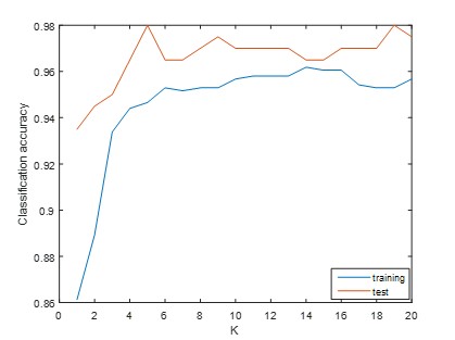
The choice of the number of neighbors K has a significant impact on the performance of SNF algorithm and subsequently influences the classification performance. To determine the optimal value of K for our classification task, we tested a range of values from 1 to 20. Figure 5 displays the classification results corresponding to different values of K. It is evident from this figure that varying values of K result in distinct classification accuracies. To strike a balance between the classification performance on the training and test dataset, we selected the value of K as 13 in current study.

3.6. Classification Performance of Different λ Values

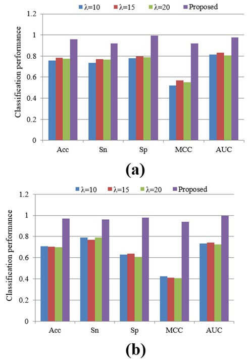
In terms of the amount of features, the value of λ is very important, which has an effect on the performance of the classification. To obtain as much information as possible, in this paper, we studied three different λ values: 10, 15 and 20. In order to investigate the performance of these various values in this subsection, we conducted additional experiments. Figure 6 shows the classification results for each λ value. Clearly, it can be observed that different λ values lead to distinct classification outcomes, both on the training and test dataset. Remarkably, our proposed method consistently surpassed the others, delivering exceptional classification performance.

3.7. Effect of Feature Selection

The main task of feature selection is in the process of eliminating redundant and irrelevant information, which can be used to enhance the classification performance. In this research, we employed the ANOVA feature selection approach to pinpoint the most discriminative features. Additionally, we compared ANOVA with other commonly used feature selection approaches, including F-score [43-47], Fisher [48, 49], and t-test [50]. The outcomes of these methods can be found in (Table 2). Table 2 shows that different feature selection approaches produce different kinds of classification performances. In comparison to the other approaches, ANOVA consistently achieved superior classification performance in terms of Acc, Sn, Sp, MCC, and AUC both on the training and test datasets.

TABLE 2: Classification performance of different feature selection methods.

Dataset	Feature selection	Acc (%)	Sn (%)	Sp (%)	MCC	AUC
Training	ANOVA	95.80	92.11	99.49	0.9185	0.9768
	Fisher	91.35	91.86	90.84	0.8270	0.9654
	F-score	76.59	87.79	65.39	0.5457	0.7786
	t-test	86.01	86.26	85.75	0.7201	0.8700
Test	ANOVA	97.00	96.00	98.00	0.9402	0.9954
	Fisher	93.50	99.00	88.00	0.8753	0.9629
	F-score	94.00	97.00	91.00	0.8816	0.9476
	t-test	90.00	83.00	97.00	0.8080	0.9294

3.8. Classification Performance of Different Classifiers

The decision made by the classifier has a big impact on the model’s classification results. In this study, we utilized SVM as the classifier for our experiments. Nevertheless, a lot of different machine learning algorithms have been used extensively in a variety of investigations, and other classifiers were used in our additional tests to examine the classification performance. Other classifiers included K nearest neighbor (KNN) [16, 43, 51], Decision Tree (DT) [52], Naïve Bayes (NB) [43, 52, 53], and Random Forest (RF) [13, 16, 43, 52, 53].

In the KNN algorithm, we compared two distance metrics: Euclidean distance (KNN-E) and cosine distance (KNN-C), using a neighbor count of 1. The RF algorithm involved using 300 decision trees. The Naïve Bayes and DT algorithms use Matlab 2015b default parameters. The outcomes of these experiments are shown in (Table 3). It can be seen from (Table 3) that SVM performed the best in both datasets and performed better than the other classifiers. In addition, SVM demonstrated a more consistent performance in comparison to the other algorithms. For example, while KNN achieved more than 90% classification accuracy on the training dataset, its accuracy on the test dataset just slightly above 70%.

TABLE 3: Classification results of different classifiers.

Dataset	Classifier	Acc (%)	Sn (%)	Sp (%)	MCC
Training	KNN-E	91.86	87.28	96.44	0.8407
	KNN-C	91.09	86.77	95.42	0.8250
	NB	93.13	89.57	96.69	0.8648
	DT	82.32	84.22	80.41	0.6468
	RF	89.82	88.55	91.09	0.7967
	SVM	95.80	92.11	99.49	0.9185
Test	KNN-E	71.00	42.00	100.00	0.5156
	KNN-C	77.50	57.00	98.00	0.6030
	NB	90.00	82.00	98.00	0.8104
	DT	74.50	74.00	75.00	0.4900
	RF	74.00	77.00	71.00	0.4809
	SVM	97.00	96.00	98.00	0.9402

3.9. Convergence of ATG-Pred Model

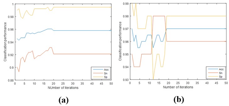
In this subsection, we performed additional analyses on the convergence of our proposed model. Figure 7 shows how the number of iterations increases of classification performance. From this figure, we can observe that the classification performance tends to stabilize around 20 iterations. It is shown that there are very few iterations in our model when it comes to convergence.

3.10. Comparison of SNF with a Hybrid Model

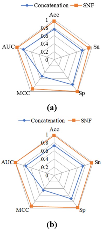
In previous studies, researchers often concatenated different feature descriptors to achieve feature fusion without considering the correlation among these features. Nevertheless, this approach overlooks the potential benefits of incorporating correlation information. In this study, we addressed this limitation by adopting the SNF algorithm to integrate different kinds of features. Figure 8 compares the classification results obtained through feature concatenation and the SNF algorithm. It is clear that a substantial gap exists between the two strategies. The SNF algorithm used in this work outperformed the direct concatenation of different features in terms of classification performance. This suggests that considering the correlation information among distinct features significantly enhances the classification task.

3.11. Comparison with the Existing Method

To further highlight the efficacy of our suggested strategy, we ran a comparison with the state-of-the-art approach. In the previous study, the model was evaluated using a 10-fold cross-validation test. Additionally, we used the same 10-fold cross-validation test to assess our approach in order to guarantee a fair comparison. A summary of the classification results is shown in (Table 4), and the mean values are shown as the metrics. It is evident from (Table 4) that ATG-Pred achieved superior classification performance both on the training and test dataset, particularly for the test dataset. For instance, the Acc and MCC for ATGPres-FL on the test dataset were reported as 90.50% and 0.810, respectively. In contrast, the proposed approach obtained higher values of 96.70% and 0.934 for these metrics on the corresponding indexes. Furthermore, the sensitivity and specificity of our method were also better than others. The efficacy of our suggested strategy for autophagy protein prediction is shown by these data.

TABLE 4: A comparison of the proposed method with the existing approach.

Dataset	Predictor	Acc (%)	Sn (%)	Sp (%)	MCC
Training	ATG-Pred-FL [22]	94.40	94.15	94.66	0.888
	ATG-Pred	95.78	92.11	99.44	0.918
Test	ATG-Pred-FL [22]	90.50	89.00	92.00	0.810
	ATG-Pred	96.70	95.30	98.10	0.934

3.12. Case Study

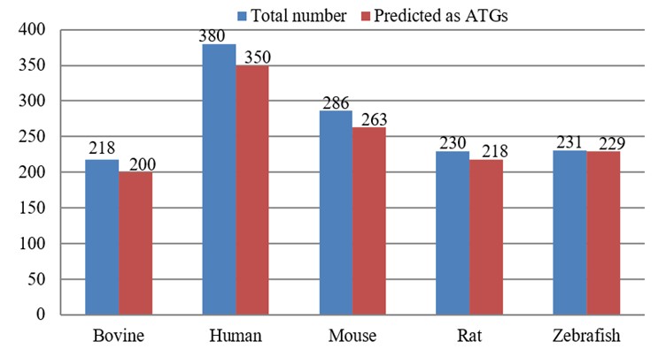
To further assess the efficacy of the proposed ATG-Pred model, we conduct experiments on a set of new ATGs from un-reviewed annotations in UniProtKB. These data were collected from a prior study [22], and they can be downloaded from the following link (Link 2). Figure 9 shows the results of these tests. From this figure, we can find that based on the predictions made by our ATG-Pred model, approximately 91.74%, 92.11%, 91.96%, 94.78%, and 99.13% of the un-reviewed protein sequences from Bovine, Human, Mouse, Rat, and Zebrafish, respectively, are predicted to be ATGs. The efficacy of our model in precisely anticipating ATGs was shown by these results.

4. Conclusion

In this study, we proposed a support vector machine based model, called ATG-Pred, for the identification of ATGs using the residue pairwise energy content. We chose an appropriate subset of features using the ANOVA feature selection method, which finally improved the model’s classification performance. Through extensive experiments using the jackknife test, our proposed method achieved high classification accuracies of 95.80% and 97.00% on the training and test datasets, respectively. Additionally, we evaluated the performance of ATG-Pred against existing predictor, and the results showed that our proposed method surpassed the state-of-the-art approach. This confirms the effectiveness of ATG-Pred in accurately identifying ATGs. To facilitate academic use, we have made the codes and datasets used in this study available at the following link (Link 3).

While ATG-Pred exhibited improved classification performance compared to prior study, it is important to acknowledge the limitations of our work. The first one is that we solely used the RECM to denote protein sequences. The RECM only capture one side of information about proteins. There are many kinds of characteristics can be used as features to denote protein. Previous studies have reported that incorporating many types of information, such as physicochemical property and evolutionary information, may enhance the performance of classification model. Therefore, future work should explore the integration of various types of information to further improve the ATG prediction accuracy of our model. Another is that we just used the correlation between two different properties, it is unknown whether interactions among more properties may benefit for improving the classification performance, we will explore this issue in the future.

Data Availability Statement

The codes and datasets used in this study were available at (Link 4).

Conflicts of Interest

None.

Acknowledgments

This work was supported by Jiangxi Provincial Natural Science Foundation (20242BAB20072), the Youth Project of Jiangxi Education Department (GJJ2201350), the Doctoral start-up fund of Jiangxi Science and Technology Normal University (2022BSQD20).The author gratefully acknowledge the partial support from the Jiangxi Science and Technology Normal University, and Jiangxi Engineering Research Center of Unattended Perception System and Artificial Intelligence Technology.

Ethical Approval

This article does not contain any studies with human participants or animals performed by any of the authors.

Informed Consent

There was no human participant and consent was not required.

REFERENCES

1.    Yu Luo, Chen Jiang, Lihua Yu, et al. “Chemical biology of autophagy-related proteins with posttranslational modifications: from chemical synthesis to biological applications. Front Chem, vol. 8, pp. 233, 2020. View at: Publisher Site | PubMed

2.    Fiona M Menzies, Angeleen Fleming, David C Rubinsztein “Compromised autophagy and neurodegenerative diseases.” Nat Rev Neurosci, vol. 16, no. 6, pp. 345-357, 2015. View at: Publisher Site | PubMed

3.    Eileen White “The role for autophagy in cancer.” J Clin Invest, vol. 125, no. 1, pp. 42-46, 2015. View at: Publisher Site | PubMed

4.    Malene Hansen, David C Rubinsztein, David W Walker “Autophagy as a promoter of longevity: insights from model organisms.” Nat Rev Mol Cell Biol, vol. 19, no. 9, pp. 579-593, 2018. View at: Publisher Site | PubMed

5.    Beth Levine, Guido Kroemer “Biological functions of autophagy genes: a disease perspective.” Cell, vol. 176, no. 1-2, pp. 11-42, 2019. View at: Publisher Site | PubMed

6.    Beth Levine, Daniel J Klionsky “Autophagy wins the 2016 Nobel Prize in Physiology or Medicine: Breakthroughs in baker's yeast fuel advances in biomedical research.” Proc Natl Acad Sci U S A, vol. 114, no. 2, pp. 201-205, 2017. View at: Publisher Site | PubMed

7.    Isei Tanida “Autophagosome formation and molecular mechanism of autophagy.” Antioxid Redox Signal, vol. 14, no. 11, pp. 2201-2214, 2011. View at: Publisher Site | PubMed

8.    Da-wei Wang, Zhen-ju Peng, Guang-fang Ren, et al. “The different roles of selective autophagic protein degradation in mammalian cells.” Oncotarget, vol. 6, no. 35, pp. 37098-37116, 2015. View at: Publisher Site | PubMed

9.    Farid Nasiri, Fereshteh Fallah Atanaki, Saman Behrouzi, et al. “CpACpP: In Silico Cell-Penetrating Anticancer Peptide Prediction Using a Novel Bioinformatics Framework.” ACS Omega, vol. 6, no. 30, pp. 19846-19859, 2021. View at: Publisher Site | PubMed

10. Jiani Ma, Lin Zhang, Jin Chen, et al. “m⁷GDisAI: N7-methylguanosine (m 7 G) sites and diseases associations inference based on heterogeneous network.” BMC Bioinformatics, vol. 22, no. 1, pp. 152, 2021. View at: Publisher Site | PubMed

11. Kewei Liu, Wei Chen “iMRM: a platform for simultaneously identifying multiple kinds of RNA modifications.” Bioinformatics, vol. 36, no. 11, pp. 3336-3342, 2020. View at: Publisher Site | PubMed

12. Bin Liu, Ren Long, Kuo-Chen Chou “iDHS-EL: identifying DNase I hypersensitive sites by fusing three different modes of pseudo nucleotide composition into an ensemble learning framework.” Bioinformatics, vol. 32, no. 16, pp. 2411-2418, 2016. View at: Publisher Site | PubMed

13. Dae Yeong Lim, Jhabindra Khanal, Hilal Tayara, “iEnhancer-RF: Identifying enhancers and their strength by enhanced feature representation using random forest.” Chemometrics and Intelligent Laboratory Systems, vol. 212, pp. 104284, 2021. View at: Publisher Site

14. Nguyen Quoc Khanh Le, Edward Kien Yee Yapp, Quang-Thai Ho, et al. “iEnhancer-5Step: identifying enhancers using hidden information of DNA sequences via Chou's 5-step rule and word embedding.” Anal Biochem, vol. 571, pp. 53-61, 2019. View at: Publisher Site | PubMed

15. Md Mehedi Hasan, Md Ashad Alam, Watshara Shoombuatong, et al. “NeuroPred-FRL: an interpretable prediction model for identifying neuropeptide using feature representation learning.” Brief Bioinform, vol. 22, no. 6, pp. bbab167, 2021. View at: Publisher Site | PubMed

16. Ruyu Dai, Wei Zhang, Wending Tang, et al. “BBPpred: sequence-based prediction of blood-brain barrier peptides with feature representation learning and logistic regression.” J Chem Inf Model, vol. 61, no. 1, pp. 525-534, 2021. View at: Publisher Site | PubMed

17. Wei Chen, Pengmian Feng, Xiaoming Song, et al. “iRNA-m7G: identifying N7-methylguanosine sites by fusing multiple features.” Mol Ther Nucleic Acids, vol. 18, pp. 269-274, 2019. View at: Publisher Site | PubMed

18. Haitao Han, Wenhong Zhu, Chenchen Ding, “iPVP-MCV: A Multi-Classifier Voting Model for the Accurate Identification of Phage Virion Proteins.” Symmetry, vol. 13, no. 8, pp. 1506, 2021. View at: Publisher Site

19. Xiaoyong Pan, Jasper Zuallaert, Xi Wang, “ToxDL: deep learning using primary structure and domain embeddings for assessing protein toxicity.” Bioinformatics, vol. 36, no. 21, pp. 5159-5168, 2020. View at: Publisher Site | PubMed

20. Xiaoyong Pan, Lei Chen, Min Liu, “Identifying protein subcellular locations with embeddings-based node2loc.” IEEE/ACM Trans Comput Biol Bioinform, vol. 19, no. 2, pp. 666-675, 2022. View at: Publisher Site | PubMed

21. Yang Lin, Xiaoyong Pan, Hong-Bin Shen “lncLocator 2.0: a cell-line-specific subcellular localization predictor for long non-coding RNAs with interpretable deep learning.” Bioinformatics, vol. 37, no. 16, pp. 2308-2316, 2021. View at: Publisher Site | PubMed

22. Shihu Jiao, Zheng Chen, Lichao Zhang, et al. “ATGPred-FL: sequence-based prediction of autophagy proteins with feature representation learning.” Amino Acids, vol. 54, no. 5, pp. 799-809, 2022. View at: Publisher Site | PubMed

23. UniProt Consortium “UniProt: the universal protein knowledgebase in 2021.” Nucleic Acids Res, vol. 49, no. D1, pp. D480-D489, 2021. View at: Publisher Site | PubMed

24. Marco Punta, Penny C Coggill, Ruth Y Eberhardt, et al. “The Pfam protein families database.” Nucleic Acids Res, vol. 40, no. D1, pp. D290-D301, 2012. View at: Publisher Site | PubMed

25. Limin Fu, Beifang Niu, Zhengwei Zhu, et al. “CD-HIT: accelerated for clustering the next-generation sequencing data.” Bioinformatics, vol. 28, no. 23, pp. 3150-3152, 2012. View at: Publisher Site | PubMed

26. Zsuzsanna Dosztányi, Veronika Csizmók, Péter Tompa, et al. “The pairwise energy content estimated from amino acid composition discriminates between folded and intrinsically unstructured proteins.” J Mol Biol, vol. 347, no. 4, pp. 827-839, 2005. View at: Publisher Site | PubMed

27. Xiangzheng Fu, Lijun Cai, Xiangxiang Zeng, et al. “StackCPPred: a stacking and pairwise energy content-based prediction of cell-penetrating peptides and their uptake efficiency.” Bioinformatics, vol. 36, no. 10, pp. 3028-3034, 2020. View at: Publisher Site | PubMed

28. Avdesh Mishra, Reecha Khanal, Wasi Ul Kabir, et al. “AIRBP: accurate identification of RNA-binding proteins using machine learning techniques.” Artif Intell Med, vol. 113, pp. 102034, 2021. View at: Publisher Site | PubMed

29. Xuan Xiao, Pu Wang, Kuo-Chen Chou “iNR-PhysChem: a sequence-based predictor for identifying nuclear receptors and their subfamilies via physical-chemical property matrix.” PLoS One, vol. 7, no. 2, pp. e30869, 2012. View at: Publisher Site | PubMed

30. Bo Wang, Aziz M Mezlini, Feyyaz Demir, et al. “Similarity network fusion for aggregating data types on a genomic scale.” Nat Methods, vol. 11, no. 3, pp. 333-337, 2014. View at: Publisher Site | PubMed

31. Hao Lin, Hui Ding “Predicting ion channels and their types by the dipeptide mode of pseudo amino acid composition.” J Theor Biol, vol. 269, no. 1, pp. 64-69, 2011. View at: Publisher Site | PubMed

32. Kuo Wang, Sumei Li, Qing Wang, et al. “Identification of hormone-binding proteins using a novel ensemble classifier.” Computing, vol. 101, no. 6, pp. 693-703, 2019. View at: Publisher Site

33. Jiu-Xin Tan, Fu-Ying Dao, Hao Lv, et al. “Identifying phage virion proteins by using two-step feature selection methods.” Molecules, vol. 23, no. 8, pp. 2000, 2018. View at: Publisher Site | PubMed

34. Xianhai Li, Qiang Tang, Hua Tang, et al. “Identifying antioxidant proteins by combining multiple methods.” Front Bioeng Biotechnol, vol. 8, pp. 858, 2020. View at: Publisher Site | PubMed

35. Balachandran Manavalan, Shaherin Basith, Tae Hwan Shin, et al. “Computational prediction of species-specific yeast DNA replication origin via iterative feature representation.” Brief Bioinform, vol. 22, no. 4, pp. bbaa304, 2021. View at: Publisher Site | PubMed

36. SiJie Yao, ChunHou Zheng, Bing Wang, et al. “A two-step ensemble learning for predicting protein hot spot residues from whole protein sequence.” Amino Acids, vol. 54, no. 5, pp. 765-776, 2022. View at: Publisher Site | PubMed

37. Wei Zhang, Enhua Xia, Ruyu Dai, et al. “PredAPP: Predicting Anti-Parasitic Peptides with Undersampling and Ensemble Approaches.” Interdiscip Sci, vol. 14, no. 1, pp. 258-268, 2022. View at: Publisher Site | PubMed

38. Saeed Ahmad, Phasit Charoenkwan, Julian M W Quinn, et al. “SCORPION is a stacking-based ensemble learning framework for accurate prediction of phage virion proteins.” Sci Rep, vol. 12, no. 1, pp. 4106, 2022. View at: Publisher Site | PubMed

39. Hao Wang, Qilemuge Xi, Pengfei Liang, et al. “IHEC_RAAC: a online platform for identifying human enzyme classes via reduced amino acid cluster strategy.” Amino Acids, vol. 53, no. 2, pp. 239-251, 2021. View at: Publisher Site | PubMed

40. Hongliang Zou, Zhijian Yin “Identifying dipeptidyl peptidase-IV inhibitory peptides based on correlation information of physicochemical properties.” Int J Pept Res Ther, vol. 27, no. 4, pp. 2651-2659, 2021. View at: Publisher Site

41. Hongliang Zou, Chun Zhan Using Multi‐Level Correlation Information to Identify Amyloidogenic Peptides. ChemistrySelect, vol. 7, no. 10, pp. e202104578, 2022. View at: Publisher Site

42. Mst Shamima Khatun, Md Mehedi Hasan, Watshara Shoombuatong, et al. “ProIn-Fuse: improved and robust prediction of proinflammatory peptides by fusing of multiple feature representations.” J Comput Aided Mol Des, vol. 34, no. 12, pp. 1229-1236, 2020. View at: Publisher Site | PubMed

43. Cangzhi Jia, Wenying He “EnhancerPred: a predictor for discovering enhancers based on the combination and selection of multiple features.” Sci Rep, vol. 6, pp. 38741, 2016. View at: Publisher Site | PubMed

44. Balachandran Manavalan, Shaherin Basith, Tae Hwan Shin, et al. “AtbPpred: A Robust Sequence-Based Prediction of Anti-Tubercular Peptides Using Extremely Randomized Trees.” Comput Struct Biotechnol J, vol. 17, pp. 972-981, 2019. View at: Publisher Site | PubMed

45. Xue Chen, Qianyue Zhang, Bowen Li, et al. “BBPpredict: A Web Service for Identifying Blood-Brain Barrier Penetrating Peptides.” Front Genet, vol. 13, pp. 845747, 2022. View at: Publisher Site | PubMed

46. Qiang Tang, Fulei Nie, Juanjuan Kang, et al.” ncPro-ML: an integrated computational tool for identifying non-coding RNA promoters in multiple species.” Comput Struct Biotechnol J, vol. 18, pp. 2445-2452, 2020. View at: Publisher Site | PubMed

47. Hui Yang, Wuritu Yang, Fu-Ying Dao, et al. “A comparison and assessment of computational method for identifying recombination hotspots in Saccharomyces cerevisiae.” Brief Bioinform, vol. 21, no. 5, pp. 1568-1580, 2020. View at: Publisher Site | PubMed

48. Ali Khazaee, Ata Ebrahimzadeh, Abbas Babajani-Feremi “Application of advanced machine learning methods on resting-state fMRI network for identification of mild cognitive impairment and Alzheimer's disease.” Brain Imaging Behav, vol. 10, no. 3, pp. 799-817, 2016. View at: Publisher Site | PubMed

49. Hongliang Zou “Identifying blood‐brain barrier peptides by using amino acids physicochemical properties and features fusion method.” Peptide Science, vol. 114, no. 2, pp. e24247, 2022. View at: Publisher Site

50. Iman Beheshti, Hasan Demirel “Feature-ranking-based Alzheimer’s disease classification from structural MRI.” Magn Reson Imaging, vol. 34, no. 3, pp. 252-263, 2016. View at: Publisher Site | PubMed

51. Yannan Bin, Wei Zhang, Wending Tang, et al. “Prediction of Neuropeptides from Sequence Information Using Ensemble Classifier and Hybrid Features.” J Proteome Res, vol. 19, no. 9, pp. 3732-3740, 2020. View at: Publisher Site | PubMed

52. Jianying Lin, Hui Chen, Shan Li, et al. “Accurate prediction of potential druggable proteins based on genetic algorithm and Bagging-SVM ensemble classifier.” Artif Intell Med, vol. 98, pp. 35-47, 2019. View at: Publisher Site | PubMed

53. Phasit Charoenkwan, Chanin Nantasenamat, Md Mehedi Hasan, et al. “Meta-iPVP: a sequence-based meta-predictor for improving the prediction of phage virion proteins using effective feature representation.” J Comput Aided Mol Des, vol. 34, no. 10, ppp. 1105-1116, 2020. View at: Publisher Site | PubMed